5. Oligoset Generation

The final step in designing oligos is to organize them into optimal sets that maximize experimental efficiency and reliability. This step evaluates individual oligos, groups them into sets of non-overlapping oligos and ranks the sets by their overall efficiency scores. The OligosetGenerator ensures that only the best-performing sets of oligos are selected for downstream experimental use.

Key Objectives in Oligoset Generation

Scoring Individual Oligos: Each oligo is assigned a score based on its theoretical efficiency in the experimental context. Scores are computed using a class derived from OligoScoringBase. A list of implemented oligo scores is available here.
Scoring Oligo Sets: Once individual oligos are scored, they are grouped into sets of oligos based on a set generator. A scoring class derived from SetScoringBase evaluates the overall efficiency of each set. A list of implemented oligo scores is available here.
Generating Oligo Sets: Oligos in each set can be selected based on their positional overlap (OligosetGeneratorIndependentSet) or the homogeneity of specified oligo properties (HomogeneousPropertyOligoSetGenerator).
Selection Policies: The OligoSelectionPolicy classes define the strategy for selecting and optimizing non-overlapping oligo sets from a pool of candidates. These policies use greedy or graph-based approaches to navigate the large combinatorial space of possible oligo combinations. This ensures the generated sets meet experimental requirements while adhering to constraints like set size and distance between oligos.

In this tutorial we show how one can:

Score oligos
Generate non-everlapping sets with a graph-based approach
Get ready-to-use oligo sets

Imports and setup

[1]:

import os
import seaborn as sns
import matplotlib.pyplot as plt

from pathlib import Path
from Bio.SeqUtils import MeltingTemp as mt

from oligo_designer_toolsuite.database import OligoDatabase
from oligo_designer_toolsuite.oligo_efficiency_filter import (
    LowestSetScoring,
    IsoformConsensusScorer,
    NormalizedDeviationFromOptimalTmScorer,
    NormalizedDeviationFromOptimalGCContentScorer,
    OligoScoring
)
from oligo_designer_toolsuite.oligo_property_calculator import (
    GCContentProperty,
    PropertyCalculator,
    TmNNProperty,
)
from oligo_designer_toolsuite.oligo_selection import (
    GraphBasedSelectionPolicy,
    OligosetGeneratorIndependentSet,
)

[2]:

dir_output = os.path.abspath("./results")
Path(dir_output).mkdir(parents=True, exist_ok=True)

n_jobs = 3

[3]:

# parameters
oligo_Tm_opt = 65
oligo_GC_content_opt = 50
oligo_isoform_weight = 2
oligo_Tm_weight = 1
oligo_GC_weight = 1

pre_filter = False
n_attempts = 100000
heuristic = True
heuristic_n_attempts = 100
clique_init_approximation = False

max_graph_size = 5000
distance_between_oligos = 0

oligo_size_opt = 5
oligo_size_min = 3
n_sets = 100

oligo_GC_content_min = 40
oligo_GC_content_max = 60

oligo_Tm_min = 60
oligo_Tm_max = 70

Tm_parameters_oligo = {
    "nn_table": "DNA_NN3", # Allawi & SantaLucia (1997)
    "tmm_table": "DNA_TMM1", #default
    "imm_table": "DNA_IMM1", #default
    "de_table": "DNA_DE1", #default
    "dnac1": 50, #[nM]
    "dnac2": 0, #[nM]
    "saltcorr": 7, # Owczarzy et al. (2008)
    "Na": 39, #[mM]
    "K": 75, #[mM]
    "Tris": 20, #[mM]
    "Mg": 10, #[mM]
    "dNTPs": 0, #[mM] default
}
Tm_parameters_oligo["nn_table"] = getattr(mt, Tm_parameters_oligo["nn_table"])
Tm_parameters_oligo["tmm_table"] = getattr(mt, Tm_parameters_oligo["tmm_table"])
Tm_parameters_oligo["imm_table"] = getattr(mt, Tm_parameters_oligo["imm_table"])
Tm_parameters_oligo["de_table"] = getattr(mt, Tm_parameters_oligo["de_table"])

Tm_chem_correction_param_oligo = {
    "DMSO": 0, #default
    "fmd": 20,
    "DMSOfactor": 0.75, #default
    "fmdfactor": 0.65, #default
    "fmdmethod": 1, #default
    "GC": None, #default
}

Load the database

Like in previous tutorials, we will also be working with OligoDatabase objects. If you don’t know how they work, please check our oligo database tutorial. In this tutorial, we will load an existing database.

[4]:

# Create Database object
min_oligos_per_region = 3
write_regions_with_insufficient_oligos = True
max_entries_in_memory=n_jobs * 2 + 2
database_name="db_oligos"

oligo_database = OligoDatabase(
    min_oligos_per_region=min_oligos_per_region,
    write_regions_with_insufficient_oligos=write_regions_with_insufficient_oligos,
    max_entries_in_memory=max_entries_in_memory,
    database_name=database_name,
    dir_output=dir_output,
    n_jobs=n_jobs,
)

# Load Database
dir_database = os.path.abspath("./data/3_db_oligos_specificity_filter")
oligo_database.load_database(dir_database=dir_database, database_overwrite=True, merge_databases_on_sequence_type="oligo")

Below we show the table of oligos for region AARS1, where we computed oligo properties like melting temperature and GC content for each oligo.

We can compare it later with the oligos that are kept after the set selection.

[5]:

properties = [
    GCContentProperty(),
    TmNNProperty(
        Tm_parameters=Tm_parameters_oligo,
        Tm_chem_correction_parameters=Tm_chem_correction_param_oligo,
        Tm_salt_correction_parameters=None,
    ),
]
calculator = PropertyCalculator(properties=properties)
oligo_database = calculator.apply(
    oligo_database=oligo_database, sequence_type="oligo", n_jobs=n_jobs
)

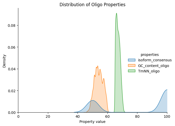
[6]:

output_table = oligo_database.get_oligo_property_table(properties=["oligo", "oligo_score", "isoform_consensus", "GC_content_oligo", "TmNN_oligo"], flatten=True, region_ids="AARS1")
output_table_plot = output_table.melt(id_vars="oligo_id", value_vars=["isoform_consensus", "GC_content_oligo", "TmNN_oligo"], var_name="properties", value_name="property_value")

sns.displot(data=output_table_plot, x="property_value", hue="properties", kind="kde", fill=True)
plt.title("Distribution of Oligo Properties")
plt.xlabel("Property value")
plt.xlim([0, 100])
plt.tight_layout()
plt.show()

../../_images/_getting_started__tutorials_5-oligoset-generation_9_0.png

Scoring

Each oligo scorer is implemented as a class inheriting from the abstract base class BaseScorer. This ensures all scorer have a standardized apply() method, which takes an OligoDatabase object, region_id and oligo_id as input and returns the calculated score. The OligoScoring class takes one or multiple scorer as inputs, iterates through a given set of region_ids and applies each scorer to the oligos of that region. The individual scores are summed for each oligo.

[ ]:

# oligo scoring
isoform_scorer = IsoformConsensusScorer(score_weight=oligo_isoform_weight)
Tm_scorer = NormalizedDeviationFromOptimalTmScorer(
    Tm_min=oligo_Tm_min,
    Tm_opt=oligo_Tm_opt,
    Tm_max=oligo_Tm_max,
    Tm_parameters=Tm_parameters_oligo,
    Tm_chem_correction_parameters=Tm_chem_correction_param_oligo,
    Tm_salt_correction_parameters=None,
    score_weight=oligo_Tm_weight,
)
GC_scorer = NormalizedDeviationFromOptimalGCContentScorer(
    GC_content_min=oligo_GC_content_min,
    GC_content_opt=oligo_GC_content_opt,
    GC_content_max=oligo_GC_content_max,
    score_weight=oligo_GC_weight,
)
oligos_scoring = OligoScoring(scorers=[isoform_scorer, Tm_scorer, GC_scorer])

# set scoring
set_scoring = LowestSetScoring(ascending=True)

Oligo Selection Policy

The GraphBasedSelectionPolicy uses the scoring strategies, defined above, to select sets of non-overlapping oligos that minimize the overall set score. Key features include:

Pre-Filtering: If pre_filter=True, oligos are pre-filtered before set selection, removing oligos that cannot form sets of at least oligo_size_min oligos. This improves performance for larger sets (e.g., oligo_size_min > 30) but can dramatically slow down small set selection (e.g., oligo_size_min < 30).

Search for Initial Set: The graph-based set selection approach starts with finding an inital set of oligos which fulfills the minimum requirements, i.e. having a size of at least oligo_size_min. If no initial set is found, the selection step is terminated for the respective region. If an initial set is found, this set is used as starting point for selecting optimal sets by minimizing the overall set score. For larger sets (e.g., oligo_size_min > 15) the prformance improves when we use an approximation that finds the largest non-overlapping set in the graph using clique_init_approximation=True, however, if the set size is small (e.g., oligo_size_min < 15) it is more efficient to iterate through all possible non-overlapping sets by setting clique_init_approximation=False.

Heuristic Search: A heuristic approach is employed to optimize set selection within a feasible runtime:

heuristic: Enables or disables heuristic optimization for faster results, which might not find the best possible set.
heuristic_n_attempts: Maximum number of attempts to find optimal sets.

Generating Oligosets

Using the OligosetGeneratorIndependentSet, the pipeline generates non-overlapping sets of oligos. The generator uses the scoring strategies and selection policies to create optimal sets of a user-defined size.

Set Parameters:

set_size_opt: Optimal number of oligos per set.
set_size_min: Minimum number of oligos required for a set.
n_sets: Number of sets to generate.

Graph Constraints:

max_graph_size: Limits the size of the graph for feasible computation.
distance_between_oligos: Ensures no overlap between selected oligos.

Note: If min_set_size is set to a large value, consider switching from the graph-based selection policy to the GreedySelectionPolicy, as it increases the likelihood of finding large sets. However, keep in mind that the greedy approach may yield lower-scoring sets compared to the graph-based method.

[8]:

selection_policy = GraphBasedSelectionPolicy(
    set_scoring=set_scoring,
    pre_filter=pre_filter,
    n_attempts=n_attempts,
    heuristic=heuristic,
    heuristic_n_attempts=heuristic_n_attempts,
    clique_init_approximation=clique_init_approximation,
)
probeset_generator = OligosetGeneratorIndependentSet(
    selection_policy=selection_policy,
    oligos_scoring=oligos_scoring,
    set_scoring=set_scoring,
    max_oligos=max_graph_size,
    distance_between_oligos=distance_between_oligos,
)

[9]:

oligo_database = probeset_generator.apply(
    oligo_database=oligo_database,
    sequence_type="oligo",
    set_size_opt=oligo_size_opt,
    set_size_min=oligo_size_min,
    n_sets=n_sets,
    n_jobs=n_jobs,
)

# Save Database
dir_database = "4_db_oligoset_selection"
oligo_database.save_database(name_database=dir_database)

[9]:

'/Users/lisasousa/Desktop/odt_projects/oligo-designer-toolsuite/tutorials/results/db_oligos/4_db_oligoset_selection'

Output Structure

The generated sets are saved in a pandas DataFrame with the following structure:

oligoset_id	oligo_0	oligo_1	oligo_2	…	oligo_n	set_score_1	set_score_2	…
0	AGRN_184	AGRN_133	AGRN_832	…	AGRN_706	0.3445	1.2332	…

oligoset_id: Identifies each oligo set.
oligo_0, oligo_1, …: Oligos in the set.
set_score_*: Scores representing the set’s efficiency.

[10]:

# Show oligosets for a specific gene
oligo_database.oligosets["AARS1"]

[10]:

	oligoset_id	oligo_0	oligo_1	oligo_2	oligo_3	oligo_4	set_score_worst	set_score_sum
0	0	AARS1::2291	AARS1::10497	AARS1::14964	AARS1::12911	AARS1::11384	0.01	0.030
1	1	AARS1::10497	AARS1::2290	AARS1::14964	AARS1::12911	AARS1::13103	0.01	0.030
2	2	AARS1::10497	AARS1::2291	AARS1::14964	AARS1::12911	AARS1::13103	0.01	0.030
3	3	AARS1::10497	AARS1::2255	AARS1::14964	AARS1::12911	AARS1::13103	0.01	0.032
4	4	AARS1::10497	AARS1::2256	AARS1::14964	AARS1::12911	AARS1::13103	0.01	0.032
5	5	AARS1::10497	AARS1::14964	AARS1::12911	AARS1::13103	AARS1::1780	0.01	0.038

We can now inspect the selected oligos below. The table shows that the selected oligos all have an isoform conses of 100% (i.e. covering all isoforms), have a GC content which equal the optimal GC content and a melting temperature very close to the optimal melting temperature.

[11]:

output_table = oligo_database.get_oligo_property_table(properties=["start", "end", "oligo", "oligo_score", "isoform_consensus", "GC_content_oligo", "TmNN_oligo"], flatten=True, region_ids="AARS1")
output_table.sort_values(by="start")

[11]:

	region_id	oligo_id	start	end	oligo	oligo_score	isoform_consensus	GC_content_oligo	TmNN_oligo
4	AARS1	AARS1::2291	70261065	70261108	CTGATCCCCCACTTTCAGGTCACCGTAGATGGTTCCAATGTGTA	0.002	100.0	50.0	65.01
3	AARS1	AARS1::2290	70261066	70261109	TGATCCCCCACTTTCAGGTCACCGTAGATGGTTCCAATGTGTAG	0.002	100.0	50.0	65.01
2	AARS1	AARS1::2256	70261100	70261143	CAATGTGTAGCACATACCCTCCTCGGACCTGAGCATTCTTCACT	0.004	100.0	50.0	65.02
1	AARS1	AARS1::2255	70261101	70261144	AATGTGTAGCACATACCCTCCTCGGACCTGAGCATTCTTCACTG	0.004	100.0	50.0	65.02
0	AARS1	AARS1::1780	70262378	70262421	AGCCTTCGTCATAGATCTGGCCTCCTTGCTCAGCATAGAAACAG	0.010	100.0	50.0	65.05
9	AARS1	AARS1::14964	70267764	70267805	CCTTCACCATGTCTGGGTCCTTCTTCAGCTCAGGAAATGCAT	0.006	100.0	50.0	65.03
8	AARS1	AARS1::13103	70270282	70270321	GGCCCATCCCTGTGTCAATGCTTTTCTTGGGAAGAGGTTT	0.010	100.0	50.0	65.05
7	AARS1	AARS1::12911	70271805	70271848	TTCCAGATCTCCAGCACATTAGGGTCGTCCTGGTTGACAAGATG	0.010	100.0	50.0	65.05
6	AARS1	AARS1::11384	70276990	70277033	AGAGCCCAGCATCTCGAAGAAGGTGTGATGATAGACATCCTTGC	0.010	100.0	50.0	65.05
5	AARS1	AARS1::10497	70282670	70282713	TGGTGGCAGACGAGTGAACATACGTATGCTCGTTCCTCTTGAAG	0.002	100.0	50.0	65.01

Applying set selection to the OligoDatabase is critical for several reasons:

Ensures Experimental Efficiency: Generates sets of high-scoring oligos, ensuring effective target binding without competition.
Customizable and Scalable: Users can tailor scoring strategies and selection policies to meet specific experimental needs.
Optimized Workflow: Pre-filtering approaches and heuristic methods enable efficient generation of high-quality oligosets, even for large datasets.

This step finalizes the pipeline by providing optimal, ready-to-use oligosets tailored to experimental requirements. These sets can then be directly integrated into downstream experimental protocols.